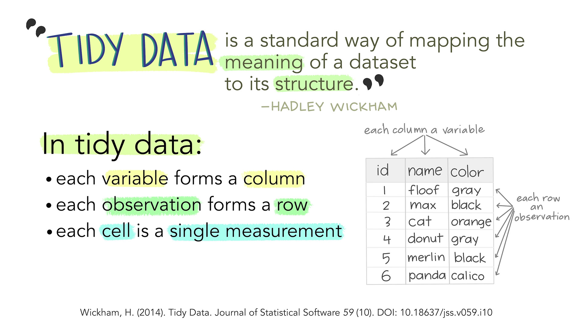
Tidy data is a way of organizing data that makes it easier to analyze and visualize. The concept of tidy data is central to the philosophy of the tidyverse.
Each variable forms a column: Each column contains all values for a single variable.
Each observation forms a row: Each row contains all values for a single observation.
Each value must have its own cell: Each cell is a single value.
Figure 6.1: Tidy data by Allison Hurst.
6.1.1 Why Tidy Data?
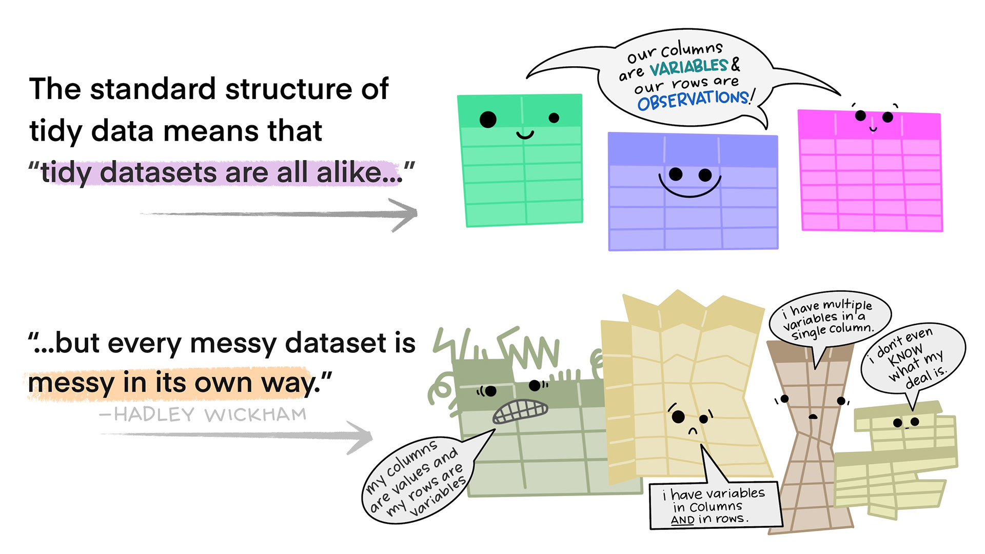
Tidy data structures are beneficial because they: - Simplify data manipulation: Functions in the tidyverse are designed to work with tidy data. Transforming, filtering, and summarizing data becomes more intuitive. - Enhance readability: Tidy data is easier to understand and interpret, making it more accessible to others. - Improve compatibility: Tidy data works seamlessly with tidyverse functions and other analytical tools.
Figure 6.2: Non-Tidy data by Allison Hurst.
According to Hadley Wickham there are five common data problems that you’ll see when analyzing a dataset:
Column headers are values, not variable names
Multiple variables are stored in one column
Variables are stored in both rows and columns
Multiple types of observational units are stored in the same table
A single observational unit is stored in multiple tables
Most of these problems can be solved with pivoting (longer and wider) and separating.
6.1.2 Example of Tidy vs. Untidy Data
Note
More examples can be found here https://tidyr.tidyverse.org/articles/tidy-data.html
In R there are over 50 built-in datasets, to see them use library(help='datasets'). We will use the Palmer penguins dataset. To use the package…
# Install and load the palmerpenguins package#install.packages("palmerpenguins")library(palmerpenguins)library(tidyverse)# Load the penguins datasetdata("penguins")# Display the first few rows of the datasethead(penguins)
species
island
bill_length_mm
bill_depth_mm
flipper_length_mm
body_mass_g
sex
year
Adelie
Torgersen
39.1
18.7
181
3750
male
2007
Adelie
Torgersen
39.5
17.4
186
3800
female
2007
Adelie
Torgersen
40.3
18.0
195
3250
female
2007
Adelie
Torgersen
NA
NA
NA
NA
NA
2007
Adelie
Torgersen
36.7
19.3
193
3450
female
2007
Adelie
Torgersen
39.3
20.6
190
3650
male
2007
The essiential tidyverse data manipulating functions can be categorized into:
Functions that provide quick insights or perform general tasks.
Examples: glimpse(), count(), arrange().
7 Data Wrangling in practice
7.1 Data integration
7.1.1 Combine multiple datasets
7.1.2 Convert data structures (e.g., pivoting between long and wide formats).
7.1.3 Merge or split variables/columns.
7.2 Data cleaning
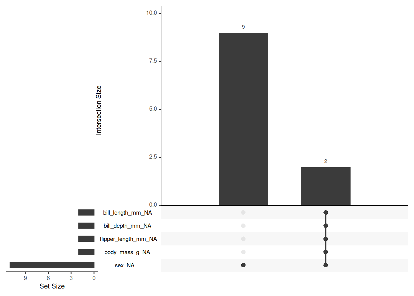
To understand if there is a pattern in the missingness you could use the gg_miss_upset()function from the package naniar.
naniar::gg_miss_upset(penguins)
And to see if the data is missing at random
misty::na.test(penguins, output=FALSE)
7.2.1 Detailed
# Load necessary librarieslibrary(dplyr)library(palmerpenguins)# Load the palmerpenguins datasetdata("penguins")# 1. Column Manipulation# mutate()# Function: Adds new variables or transforms existing ones.# Example: Add a new column 'Bill_Ratio' which is the ratio of bill length to bill depth.penguins %>%mutate(Bill_Ratio = bill_length_mm / bill_depth_mm) %>%head()
species
island
bill_length_mm
bill_depth_mm
flipper_length_mm
body_mass_g
sex
year
Bill_Ratio
Adelie
Torgersen
39.1
18.7
181
3750
male
2007
2.090909
Adelie
Torgersen
39.5
17.4
186
3800
female
2007
2.270115
Adelie
Torgersen
40.3
18.0
195
3250
female
2007
2.238889
Adelie
Torgersen
NA
NA
NA
NA
NA
2007
NA
Adelie
Torgersen
36.7
19.3
193
3450
female
2007
1.901554
Adelie
Torgersen
39.3
20.6
190
3650
male
2007
1.907767
# select()# Function: Selects columns by their names.# Example: Select only the columns 'species', 'island', 'bill_length_mm', and 'bill_depth_mm'.penguins %>%select(species, island, bill_length_mm, bill_depth_mm) %>%head()
species
island
bill_length_mm
bill_depth_mm
Adelie
Torgersen
39.1
18.7
Adelie
Torgersen
39.5
17.4
Adelie
Torgersen
40.3
18.0
Adelie
Torgersen
NA
NA
Adelie
Torgersen
36.7
19.3
Adelie
Torgersen
39.3
20.6
# rename()# Function: Renames columns.# Example: Rename 'bill_length_mm' to 'BillLength' and 'bill_depth_mm' to 'BillDepth'.penguins %>%rename(BillLength = bill_length_mm, BillDepth = bill_depth_mm) %>%head()
species
island
BillLength
BillDepth
flipper_length_mm
body_mass_g
sex
year
Adelie
Torgersen
39.1
18.7
181
3750
male
2007
Adelie
Torgersen
39.5
17.4
186
3800
female
2007
Adelie
Torgersen
40.3
18.0
195
3250
female
2007
Adelie
Torgersen
NA
NA
NA
NA
NA
2007
Adelie
Torgersen
36.7
19.3
193
3450
female
2007
Adelie
Torgersen
39.3
20.6
190
3650
male
2007
# summarise()# Function: Summarizes multiple values to a single value per group.# Example: Calculate the mean of 'bill_length_mm'.penguins %>%summarise(Mean_Bill_Length =mean(bill_length_mm, na.rm =TRUE)) %>%head()
Mean_Bill_Length
43.92193
# relocate()# Function: Changes the position of columns.# Example: Move the 'species' column to be the first column in the dataset.penguins %>%relocate(species, .before = bill_length_mm) %>%head()
island
species
bill_length_mm
bill_depth_mm
flipper_length_mm
body_mass_g
sex
year
Torgersen
Adelie
39.1
18.7
181
3750
male
2007
Torgersen
Adelie
39.5
17.4
186
3800
female
2007
Torgersen
Adelie
40.3
18.0
195
3250
female
2007
Torgersen
Adelie
NA
NA
NA
NA
NA
2007
Torgersen
Adelie
36.7
19.3
193
3450
female
2007
Torgersen
Adelie
39.3
20.6
190
3650
male
2007
# 2. Row Manipulation# filter()# Function: Only retain specific rows of data that meet the specified requirement(s).# Example: Only display data where the species is "Adelie".penguins %>%filter(species =="Adelie") %>%head()
species
island
bill_length_mm
bill_depth_mm
flipper_length_mm
body_mass_g
sex
year
Adelie
Torgersen
39.1
18.7
181
3750
male
2007
Adelie
Torgersen
39.5
17.4
186
3800
female
2007
Adelie
Torgersen
40.3
18.0
195
3250
female
2007
Adelie
Torgersen
NA
NA
NA
NA
NA
2007
Adelie
Torgersen
36.7
19.3
193
3450
female
2007
Adelie
Torgersen
39.3
20.6
190
3650
male
2007
# Example: Only display data where the species is "Adelie" or "Gentoo" and the bill length is greater than 40.penguins %>%filter(species %in%c("Adelie", "Gentoo"), bill_length_mm >40) %>%head()
species
island
bill_length_mm
bill_depth_mm
flipper_length_mm
body_mass_g
sex
year
Adelie
Torgersen
40.3
18.0
195
3250
female
2007
Adelie
Torgersen
42.0
20.2
190
4250
NA
2007
Adelie
Torgersen
41.1
17.6
182
3200
female
2007
Adelie
Torgersen
42.5
20.7
197
4500
male
2007
Adelie
Torgersen
46.0
21.5
194
4200
male
2007
Adelie
Biscoe
40.6
18.6
183
3550
male
2007
# Example: Only display data where the species is not "Adelie".penguins %>%filter(species !="Adelie") %>%head()
species
island
bill_length_mm
bill_depth_mm
flipper_length_mm
body_mass_g
sex
year
Gentoo
Biscoe
46.1
13.2
211
4500
female
2007
Gentoo
Biscoe
50.0
16.3
230
5700
male
2007
Gentoo
Biscoe
48.7
14.1
210
4450
female
2007
Gentoo
Biscoe
50.0
15.2
218
5700
male
2007
Gentoo
Biscoe
47.6
14.5
215
5400
male
2007
Gentoo
Biscoe
46.5
13.5
210
4550
female
2007
# slice()# Function: Selects rows by position.# Example: Select the first 10 rows of the dataset.penguins %>%slice(1:10)
species
island
bill_length_mm
bill_depth_mm
flipper_length_mm
body_mass_g
sex
year
Adelie
Torgersen
39.1
18.7
181
3750
male
2007
Adelie
Torgersen
39.5
17.4
186
3800
female
2007
Adelie
Torgersen
40.3
18.0
195
3250
female
2007
Adelie
Torgersen
NA
NA
NA
NA
NA
2007
Adelie
Torgersen
36.7
19.3
193
3450
female
2007
Adelie
Torgersen
39.3
20.6
190
3650
male
2007
Adelie
Torgersen
38.9
17.8
181
3625
female
2007
Adelie
Torgersen
39.2
19.6
195
4675
male
2007
Adelie
Torgersen
34.1
18.1
193
3475
NA
2007
Adelie
Torgersen
42.0
20.2
190
4250
NA
2007
# arrange()# Function: Orders rows by the values of columns.# Example: Order rows by 'bill_length_mm' in ascending order.penguins %>%arrange(bill_length_mm) %>%head()
species
island
bill_length_mm
bill_depth_mm
flipper_length_mm
body_mass_g
sex
year
Adelie
Dream
32.1
15.5
188
3050
female
2009
Adelie
Dream
33.1
16.1
178
2900
female
2008
Adelie
Torgersen
33.5
19.0
190
3600
female
2008
Adelie
Dream
34.0
17.1
185
3400
female
2008
Adelie
Torgersen
34.1
18.1
193
3475
NA
2007
Adelie
Torgersen
34.4
18.4
184
3325
female
2007
# distinct()# Function: Returns unique rows based on selected columns.# Example: Return unique combinations of 'species' and 'island'.penguins %>%distinct(species, island) %>%head()
species
island
Adelie
Torgersen
Adelie
Biscoe
Adelie
Dream
Gentoo
Biscoe
Chinstrap
Dream
# slice_sample()# Function: Randomly selects rows.# Example: Randomly select 10 rows from the dataset.penguins %>%slice_sample(n =10)
species
island
bill_length_mm
bill_depth_mm
flipper_length_mm
body_mass_g
sex
year
Adelie
Biscoe
42.7
18.3
196
4075
male
2009
Adelie
Dream
39.6
18.8
190
4600
male
2007
Adelie
Torgersen
42.0
20.2
190
4250
NA
2007
Gentoo
Biscoe
46.4
15.0
216
4700
female
2008
Chinstrap
Dream
42.4
17.3
181
3600
female
2007
Adelie
Torgersen
37.3
20.5
199
3775
male
2009
Adelie
Dream
34.0
17.1
185
3400
female
2008
Gentoo
Biscoe
44.4
17.3
219
5250
male
2008
Gentoo
Biscoe
45.5
13.7
214
4650
female
2007
Chinstrap
Dream
47.6
18.3
195
3850
female
2008
# 3. Grouping and Aggregation# group_by()# Function: Groups data by one or more variables.# Example: Group by 'species' to perform operations within each species.penguins %>%group_by(species) %>%head()
species
island
bill_length_mm
bill_depth_mm
flipper_length_mm
body_mass_g
sex
year
Adelie
Torgersen
39.1
18.7
181
3750
male
2007
Adelie
Torgersen
39.5
17.4
186
3800
female
2007
Adelie
Torgersen
40.3
18.0
195
3250
female
2007
Adelie
Torgersen
NA
NA
NA
NA
NA
2007
Adelie
Torgersen
36.7
19.3
193
3450
female
2007
Adelie
Torgersen
39.3
20.6
190
3650
male
2007
# summarise()# Function: Creates summary statistics within groups.# Example: Calculate the mean and standard deviation of 'flipper_length_mm' for each species.penguins %>%group_by(species) %>%summarise(Mean_Flipper_Length =mean(flipper_length_mm, na.rm =TRUE),SD_Flipper_Length =sd(flipper_length_mm, na.rm =TRUE),Count =n()) %>%ungroup() %>%head()
species
Mean_Flipper_Length
SD_Flipper_Length
Count
Adelie
189.9536
6.539457
152
Chinstrap
195.8235
7.131894
68
Gentoo
217.1870
6.484976
124
# ungroup()# Function: Removes grouping.# Example: Always use ungroup() after grouping to avoid errors in future calculations.penguins %>%group_by(species) %>%summarise(Mean_Flipper_Length =mean(flipper_length_mm, na.rm =TRUE)) %>%ungroup() %>%head()
species
Mean_Flipper_Length
Adelie
189.9536
Chinstrap
195.8235
Gentoo
217.1870
# Example of when ungroup() matters# Without ungroup()penguins %>%group_by(species) %>%mutate(mean_flipper_length =mean(flipper_length_mm, na.rm =TRUE)) %>%mutate(mean_body_mass =mean(body_mass_g, na.rm =TRUE)) %>%head()
species
island
bill_length_mm
bill_depth_mm
flipper_length_mm
body_mass_g
sex
year
mean_flipper_length
mean_body_mass
Adelie
Torgersen
39.1
18.7
181
3750
male
2007
189.9536
3700.662
Adelie
Torgersen
39.5
17.4
186
3800
female
2007
189.9536
3700.662
Adelie
Torgersen
40.3
18.0
195
3250
female
2007
189.9536
3700.662
Adelie
Torgersen
NA
NA
NA
NA
NA
2007
189.9536
3700.662
Adelie
Torgersen
36.7
19.3
193
3450
female
2007
189.9536
3700.662
Adelie
Torgersen
39.3
20.6
190
3650
male
2007
189.9536
3700.662
# With ungroup() in the correct placepenguins %>%group_by(species) %>%mutate(mean_flipper_length =mean(flipper_length_mm, na.rm =TRUE)) %>%ungroup() %>%mutate(mean_body_mass =mean(body_mass_g, na.rm =TRUE)) %>%head()
species
island
bill_length_mm
bill_depth_mm
flipper_length_mm
body_mass_g
sex
year
mean_flipper_length
mean_body_mass
Adelie
Torgersen
39.1
18.7
181
3750
male
2007
189.9536
4201.754
Adelie
Torgersen
39.5
17.4
186
3800
female
2007
189.9536
4201.754
Adelie
Torgersen
40.3
18.0
195
3250
female
2007
189.9536
4201.754
Adelie
Torgersen
NA
NA
NA
NA
NA
2007
189.9536
4201.754
Adelie
Torgersen
36.7
19.3
193
3450
female
2007
189.9536
4201.754
Adelie
Torgersen
39.3
20.6
190
3650
male
2007
189.9536
4201.754
# 4. Joining and Merging Data# Create a dummy dataset for joining examplesisland_info <-tibble(island =unique(penguins$island),region =c("Antarctica", "Antarctica", "Antarctica")) %>%head()# inner_join()# Function: Joins two data frames by common columns.# Example: Join the penguins dataset with island_info on the 'island' column.penguins %>%inner_join(island_info, by ="island") %>%head()
species
island
bill_length_mm
bill_depth_mm
flipper_length_mm
body_mass_g
sex
year
region
Adelie
Torgersen
39.1
18.7
181
3750
male
2007
Antarctica
Adelie
Torgersen
39.5
17.4
186
3800
female
2007
Antarctica
Adelie
Torgersen
40.3
18.0
195
3250
female
2007
Antarctica
Adelie
Torgersen
NA
NA
NA
NA
NA
2007
Antarctica
Adelie
Torgersen
36.7
19.3
193
3450
female
2007
Antarctica
Adelie
Torgersen
39.3
20.6
190
3650
male
2007
Antarctica
# left_join()# Function: Keeps all rows from the left data frame and matches with the right.# Example: Left join the penguins dataset with island_info on the 'island' column.penguins %>%left_join(island_info, by ="island") %>%head()
species
island
bill_length_mm
bill_depth_mm
flipper_length_mm
body_mass_g
sex
year
region
Adelie
Torgersen
39.1
18.7
181
3750
male
2007
Antarctica
Adelie
Torgersen
39.5
17.4
186
3800
female
2007
Antarctica
Adelie
Torgersen
40.3
18.0
195
3250
female
2007
Antarctica
Adelie
Torgersen
NA
NA
NA
NA
NA
2007
Antarctica
Adelie
Torgersen
36.7
19.3
193
3450
female
2007
Antarctica
Adelie
Torgersen
39.3
20.6
190
3650
male
2007
Antarctica
# right_join()# Function: Keeps all rows from the right data frame and matches with the left.# Example: Right join the penguins dataset with island_info on the 'island' column.penguins %>%right_join(island_info, by ="island") %>%head()
species
island
bill_length_mm
bill_depth_mm
flipper_length_mm
body_mass_g
sex
year
region
Adelie
Torgersen
39.1
18.7
181
3750
male
2007
Antarctica
Adelie
Torgersen
39.5
17.4
186
3800
female
2007
Antarctica
Adelie
Torgersen
40.3
18.0
195
3250
female
2007
Antarctica
Adelie
Torgersen
NA
NA
NA
NA
NA
2007
Antarctica
Adelie
Torgersen
36.7
19.3
193
3450
female
2007
Antarctica
Adelie
Torgersen
39.3
20.6
190
3650
male
2007
Antarctica
# full_join()# Function: Keeps all rows from both data frames.# Example: Full join the penguins dataset with island_info on the 'island' column.penguins %>%full_join(island_info, by ="island") %>%head()
species
island
bill_length_mm
bill_depth_mm
flipper_length_mm
body_mass_g
sex
year
region
Adelie
Torgersen
39.1
18.7
181
3750
male
2007
Antarctica
Adelie
Torgersen
39.5
17.4
186
3800
female
2007
Antarctica
Adelie
Torgersen
40.3
18.0
195
3250
female
2007
Antarctica
Adelie
Torgersen
NA
NA
NA
NA
NA
2007
Antarctica
Adelie
Torgersen
36.7
19.3
193
3450
female
2007
Antarctica
Adelie
Torgersen
39.3
20.6
190
3650
male
2007
Antarctica
# 5. Reshaping Data# pivot_longer()# Function: Converts wide data to long format.# Example: Convert the penguins dataset from wide to long format, focusing on bill measurements.penguins %>%pivot_longer(cols =starts_with("bill"), names_to ="Measurement", values_to ="Value") %>%head()
species
island
flipper_length_mm
body_mass_g
sex
year
Measurement
Value
Adelie
Torgersen
181
3750
male
2007
bill_length_mm
39.1
Adelie
Torgersen
181
3750
male
2007
bill_depth_mm
18.7
Adelie
Torgersen
186
3800
female
2007
bill_length_mm
39.5
Adelie
Torgersen
186
3800
female
2007
bill_depth_mm
17.4
Adelie
Torgersen
195
3250
female
2007
bill_length_mm
40.3
Adelie
Torgersen
195
3250
female
2007
bill_depth_mm
18.0
# pivot_wider()# Function: Converts long data to wide format.# Example: Convert the penguins dataset from long back to wide format.penguins_long <- penguins %>%pivot_longer(cols =starts_with("bill"), names_to ="Measurement", values_to ="Value") %>%head()penguins_long %>%pivot_wider(names_from = Measurement, values_from = Value) %>%head()
species
island
flipper_length_mm
body_mass_g
sex
year
bill_length_mm
bill_depth_mm
Adelie
Torgersen
181
3750
male
2007
39.1
18.7
Adelie
Torgersen
186
3800
female
2007
39.5
17.4
Adelie
Torgersen
195
3250
female
2007
40.3
18.0
# 6. Handling Missing Data# drop_na()# Function: Removes rows with missing values.# Example: Remove any rows that have missing values.penguins %>%drop_na() %>%head()
species
island
bill_length_mm
bill_depth_mm
flipper_length_mm
body_mass_g
sex
year
Adelie
Torgersen
39.1
18.7
181
3750
male
2007
Adelie
Torgersen
39.5
17.4
186
3800
female
2007
Adelie
Torgersen
40.3
18.0
195
3250
female
2007
Adelie
Torgersen
36.7
19.3
193
3450
female
2007
Adelie
Torgersen
39.3
20.6
190
3650
male
2007
Adelie
Torgersen
38.9
17.8
181
3625
female
2007
# replace_na()# Function: Replaces missing values with specified values.# Example: Replace missing values in 'bill_length_mm' with 0.penguins %>%replace_na(list(bill_length_mm =0)) %>%head()
species
island
bill_length_mm
bill_depth_mm
flipper_length_mm
body_mass_g
sex
year
Adelie
Torgersen
39.1
18.7
181
3750
male
2007
Adelie
Torgersen
39.5
17.4
186
3800
female
2007
Adelie
Torgersen
40.3
18.0
195
3250
female
2007
Adelie
Torgersen
0.0
NA
NA
NA
NA
2007
Adelie
Torgersen
36.7
19.3
193
3450
female
2007
Adelie
Torgersen
39.3
20.6
190
3650
male
2007
# is.na()# Function: Identifies missing values.# Example: Add a new column indicating whether the 'bill_length_mm' values are missing.penguins %>%mutate(Missing_Bill_Length =is.na(bill_length_mm)) %>%head()
species
island
bill_length_mm
bill_depth_mm
flipper_length_mm
body_mass_g
sex
year
Missing_Bill_Length
Adelie
Torgersen
39.1
18.7
181
3750
male
2007
FALSE
Adelie
Torgersen
39.5
17.4
186
3800
female
2007
FALSE
Adelie
Torgersen
40.3
18.0
195
3250
female
2007
FALSE
Adelie
Torgersen
NA
NA
NA
NA
NA
2007
TRUE
Adelie
Torgersen
36.7
19.3
193
3450
female
2007
FALSE
Adelie
Torgersen
39.3
20.6
190
3650
male
2007
FALSE
# 7. Utility Functions# glimpse()# Function: Provides a compact view of the data.# Example: Get a brief overview of the penguins dataset.glimpse(penguins) %>%data.frame() %>%head()
# count()# Function: Counts the number of occurrences of unique values.# Example: Count the number of occurrences of each species.penguins %>%count(species) %>%head()
species
n
Adelie
152
Chinstrap
68
Gentoo
124
# arrange()# Function: Orders rows by the values of columns.# Example: Order rows by 'bill_length_mm' in ascending order.penguins %>%arrange(bill_length_mm) %>%head()
species
island
bill_length_mm
bill_depth_mm
flipper_length_mm
body_mass_g
sex
year
Adelie
Dream
32.1
15.5
188
3050
female
2009
Adelie
Dream
33.1
16.1
178
2900
female
2008
Adelie
Torgersen
33.5
19.0
190
3600
female
2008
Adelie
Dream
34.0
17.1
185
3400
female
2008
Adelie
Torgersen
34.1
18.1
193
3475
NA
2007
Adelie
Torgersen
34.4
18.4
184
3325
female
2007
# Additional Functions: if_else() and case_when()# if_else()# Function: Vectorized conditional transformation.# Example: Add a new column 'Bill_Category' based on the length of the bill.penguins %>%mutate(Bill_Category =if_else(bill_length_mm >40, "Large", "Small")) %>%head()
species
island
bill_length_mm
bill_depth_mm
flipper_length_mm
body_mass_g
sex
year
Bill_Category
Adelie
Torgersen
39.1
18.7
181
3750
male
2007
Small
Adelie
Torgersen
39.5
17.4
186
3800
female
2007
Small
Adelie
Torgersen
40.3
18.0
195
3250
female
2007
Large
Adelie
Torgersen
NA
NA
NA
NA
NA
2007
NA
Adelie
Torgersen
36.7
19.3
193
3450
female
2007
Small
Adelie
Torgersen
39.3
20.6
190
3650
male
2007
Small
# case_when()# Function: Multiple conditional transformations.# Example: Add a new column 'Bill_Category' with multiple conditions.penguins %>%mutate(Bill_Category =case_when( bill_length_mm >40~"Large", bill_length_mm <=40~"Small",TRUE~"Unknown" )) %>%head()
Use version control systems like Git to track changes and collaborate with others.
8Reading in Packages
To begin any data analysis project in R, you need to load the necessary packages. These packages contain functions and datasets that facilitate data manipulation, visualization, and analysis. For example, the tidyverse package is a collection of R packages designed for data science.
# Install necessary packages if not already installedinstall.packages(c("tidyverse", "here"))# Load the necessary packageslibrary(tidyverse)library(here)
Sometimes, you may want to use a specific function from a package without loading the entire package. You can do this using the :: operator. For example, if you only need the here() function from the here package, you can use it directly as follows:
here::here()
here is the package and using the :: will call a function in that package in this case here().
9Reading in Rectangular Data
Importing data from various sources into R is a crucial step in any data analysis workflow. Rectangular data, typically stored in formats like CSV, Excel, or databases, can be easily imported using various R packages.
The here package is particularly useful for constructing file paths in a reproducible way, ensuring that your code works across different environments.
9.0.1 Importing Data with Common R Packages
9.0.1.1 Using readr for CSV Files
The readr package is part of the tidyverse and is used for reading delimited files such as CSV. In Sweden, it’s common to use commas (,) or semicolons (;) as delimiters.
library(readr)library(here)# Reading a CSV file with commas as delimitersdata_comma <-read_csv(here::here("data", "data_comma.csv"))# Reading a CSV file with semicolons as delimitersdata_semicolon <-read_csv2(here::here("data", "data_semicolon.csv"))
9.0.2 Using haven for SPSS, Stata, and SAS Files
The haven package is useful for reading data from statistical software formats such as SPSS, Stata, and SAS.
library(haven)# Reading an SPSS filedata_spss <-read_sav(here::here("data", "data_spss.sav"))# Reading a Stata filedata_stata <-read_dta(here::here("data", "data_stata.dta"))# Reading a SAS filedata_sas <-read_sas(here::here("data", "data_sas.sas"))
9.0.3 Using openxlsx for Excel Files
The openxlsx package provides a way to read Excel files, which are commonly used for data storage.
library(openxlsx)# Reading an Excel filedata_excel <-read.xlsx(here::here("data", "data_excel.xlsx"))
10Data Cleaning
Handle missing values, correct data types, and clean up data to ensure it is ready for analysis.
Save the cleaned data.
11Data Exploration
Perform initial exploration of the data to understand its structure and main characteristics (e.g., summary statistics, data visualization).
Create initial visualizations and tables to summarize data.
Manipulate and transform the data as needed for analysis (e.g., filtering, mutating, summarizing). data transformation
13Data Analysis and Visualization
Apply statistical methods to analyze the data and test hypotheses (e.g., regression analysis, t-tests).
Create detailed visualizations to explore data patterns and support analysis (e.g., scatter plots, histograms).
Generate tables to summarize statistical findings.
14Reporting Results
Document the analysis and create comprehensive reports or presentations to communicate findings (e.g., using R Markdown or Quarto).
Include visualizations and tables to illustrate key points and findings.
15Saving Data
Save the final transformed and analyzed data to a file or database for future use or sharing.
15.1 Coding best practices
Coding best practices, involves following guidelines and principles that make your code more readable, maintainable, and reproducible. Here are some key aspects of good code conduct in the context of data analysis with R:
15.1.1 Readable and Descriptive Code
Use clear and descriptive variable and function names.
Write comments to explain complex logic and steps.